Note
Go to the end to download the full example code.
Display an Isocurve#
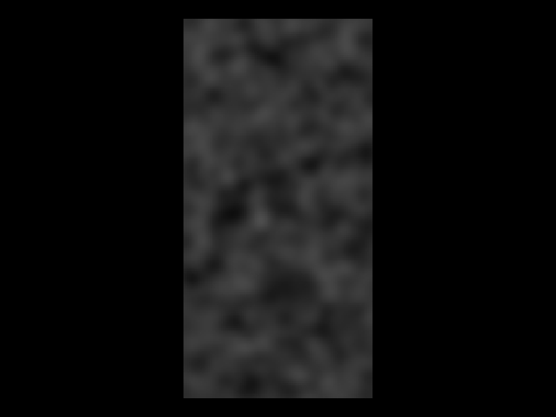
Simple use of SceneCanvas to display an Isocurve visual.

import sys
from vispy import app, scene, visuals
from vispy.util.filter import gaussian_filter
import numpy as np

canvas = scene.SceneCanvas(keys='interactive', title='Isocurve(s) overlayed '
                           'over Random Image Example')
canvas.size = 800, 600
canvas.show()

# Set up a viewbox to display the image with interactive pan/zoom
view = canvas.central_widget.add_view()

# Create the image
img_data = np.empty((200, 100, 3), dtype=np.ubyte)
noise = np.random.normal(size=(200, 100), loc=50, scale=150)
noise = gaussian_filter(noise, (4, 4, 0))
img_data[:] = noise[..., np.newaxis]
image = scene.visuals.Image(img_data, parent=view.scene)
# move image behind curves
image.transform = visuals.transforms.STTransform(translate=(0, 0, 0.5))

# level and color setup
levels = [40, 50, 60]
color_lev = [(1, 0, 0, 1),
             (1, 0.5, 0, 1),
             (1, 1, 0, 1)]

# Create isocurve, make a child of the image to ensure the two are always
# aligned.
curve = scene.visuals.Isocurve(noise, levels=levels, color_lev=color_lev,
                               parent=view.scene)

# Set 2D camera
view.camera = scene.PanZoomCamera(aspect=1)
# the camera will scale to the contents in the scene
view.camera.set_range()

if __name__ == '__main__' and sys.flags.interactive == 0:
    app.run()
Total running time of the script: (0 minutes 0.717 seconds)
